Single FID Example

This example shows an overview of the basic functionality of the Blackchirp python module. It uses data acquired using the UC Davis Ka band (26.5 - 40 GHz) CP-FTMW spectrometer.

To get started, first ensure that the module has been installed with pip install blackchirp. It is recommended to import the main blackchirp classes with from blackchirp import *. The cell below is configured to import from the development version of the module if this example notebook is run from the blackchirp source directory.

from blackchirp.src.blackchirp import * # replace with from blackchirp import *
from matplotlib import pyplot as plt

Loading and Inspecting an Experiment

In this example, we will use a CP-FTMW spectrum of methyl tert-butyl ether, which is assumed to be in the directory example-data/mtbe. This directory contains the contents of the Blackchirp data, which was copied from the original data storage location.

ll example-data/mtbe/

total 40
-rw-r--r-- 1 kncrabtree 1110 Jun  4 16:42 auxdata.csv
-rw-r--r-- 1 kncrabtree  663 Jun  4 16:42 chirps.csv
-rw-r--r-- 1 kncrabtree  127 Jun  4 16:42 clocks.csv
drwxr-xr-x 2 kncrabtree 4096 Jun  4 16:42 fid/
-rw-r--r-- 1 kncrabtree  118 Jun  4 16:42 hardware.csv
-rw-r--r-- 1 kncrabtree 7285 Jun  4 16:42 header.csv
-rw-r--r-- 1 kncrabtree  183 Jun  4 16:42 log.csv
-rw-r--r-- 1 kncrabtree   27 Jun  4 16:42 objectives.csv
-rw-r--r-- 1 kncrabtree  118 Jun  4 16:42 version.csv

The BCExperiment class is used to read in these files and construct python objects for them. Since all Blackchirp data is written in CSV format, the files are read in using pandas.read_csv and are available as pandas DataFrame objects with the same name as the corresponding CSV file. To load an experiment, pass the appropriate path to BCExperiment. This path should be the folder which contains the version.csv file for the desired experiment. Once loaded, the contents of the csv files may be inspected easily. Here we show the header.

exp = BCExperiment('./example-data/mtbe/')

exp.header

	ObjKey	ArrayKey	ArrayIndex	ValueKey	Value	Units
0	ChirpConfig		<NA>	ChirpInterval	20	μs
1	ChirpConfig		<NA>	PostGate	-0.17	μs
2	ChirpConfig		<NA>	PostProtection	0.15	μs
3	ChirpConfig		<NA>	PreGate	0.5	μs
4	ChirpConfig		<NA>	PreProtection	0.1	μs
...	...	...	...	...	...	...
176	RfConfig		<NA>	CommonUpDownLO	false
177	RfConfig		<NA>	DownconversionSideband	LowerSideband
178	RfConfig		<NA>	ShotsPerClockConfig	0
179	RfConfig		<NA>	TargetSweeps	1
180	RfConfig		<NA>	UpconversionSideband	LowerSideband

181 rows × 6 columns

Just like in the header.csv file itself, each entry is associated with an ObjKey and a ValueKey, and in some cases also an ArrayKey and ArrayIndex. The combination of these 4 values can be used to select any particular row, as shown in more detail below. Each entry has a Value and Units associated with it.

For such a large DataFrame, Jupyter notebooks typically compress the output. To get a brief overview of what information is available, use the BCExperiment.header_unique_keys() function, which returns a set containing the unique keys in the table.

exp.header_unique_keys?

Signature: exp.header_unique_keys() -> 'set[str]'
Docstring:
Fetch all unique ObjKeys in experiment header

Returns:
    List of unique header keys
File:      ~/github/blackchirp/src/python/blackchirp/src/blackchirp/blackchirpexperiment.py
Type:      method

exp.header_unique_keys()

{'ChirpConfig',
 'Experiment',
 'FtmwConfig',
 'FtmwDigitizer.0',
 'PulseGenerator.0',
 'PulseGenerator.1',
 'RfConfig'}

To view only data associated with one of these keys, use the BCExperiment.header_rows() function:

exp.header_rows?

Signature:
exp.header_rows(
    objKey: 'str' = None,
    valKey: 'str' = None,
    arrKey: 'str' = None,
) -> 'pd.DataFrame'
Docstring:
Fetch rows from the header file matching conditions

Filters rows in the header according to ObjKey, ValueKey, and ArrayKey.
Any combination of these (or none) may be specified to filter.

Args:
    objKey: Object key in header
    valKey: Value key in header
    arrKey: Array key in header

Returns:
    DataFrame with matching wors
File:      ~/github/blackchirp/src/python/blackchirp/src/blackchirp/blackchirpexperiment.py
Type:      method

For instance, to obtain only the settings related to the Pulse Generator:

exp.header_rows('PulseGenerator.0')

	ObjKey	ArrayKey	ArrayIndex	ValueKey	Value	Units
48	PulseGenerator.0		<NA>	PulseGenEnabled	true
49	PulseGenerator.0		<NA>	PulseGenMode	Triggered_Rising
50	PulseGenerator.0		<NA>	RepRate	5	Hz
51	PulseGenerator.0	Channel	0	ActiveLevel	ActiveHigh
52	PulseGenerator.0	Channel	0	Delay	0	μs
...	...	...	...	...	...	...
126	PulseGenerator.0	Channel	7	Mode	Normal
127	PulseGenerator.0	Channel	7	Name	Ch8
128	PulseGenerator.0	Channel	7	Role	None
129	PulseGenerator.0	Channel	7	SyncChannel	0
130	PulseGenerator.0	Channel	7	Width	1	μs

83 rows × 6 columns

To see only the pulse widths:

exp.header_rows('PulseGenerator.0','Width')

	ObjKey	ArrayKey	ArrayIndex	ValueKey	Value	Units
60	PulseGenerator.0	Channel	0	Width	650	μs
70	PulseGenerator.0	Channel	1	Width	150	μs
80	PulseGenerator.0	Channel	2	Width	20	μs
90	PulseGenerator.0	Channel	3	Width	2.019	μs
100	PulseGenerator.0	Channel	4	Width	1	μs
110	PulseGenerator.0	Channel	5	Width	1	μs
120	PulseGenerator.0	Channel	6	Width	1	μs
130	PulseGenerator.0	Channel	7	Width	1	μs

And finally, the BCExperiment.header_value() function retrieves one particular value from the table. A corresponding BCExperiment.header_unit() function can be used to retrieve the unit, if desired. Note that the value is returned as a string, so it may need to be explicitly cast to an int or float if the value will be used in a calculation.

exp.header_value?

Signature:
exp.header_value(
    objKey: 'str',
    valKey: 'str',
    idx: 'int' = 0,
    arrKey: 'str' = None,
) -> 'str'
Docstring:
Fetch one value from header

The objKey and valKey (and arrKey, if specified) are used to filter the header.
Then the idx value is used to determine which row to return. If a match is not
found, an empty string is returned

Args:
    objKey: Object key in header
    valKey: Value key in header
    idx: Row number to return (optional)
    arrKey: Array key in header (optional)

Returns:
    Matching value or empty string
File:      ~/github/blackchirp/src/python/blackchirp/src/blackchirp/blackchirpexperiment.py
Type:      method

exp.header_value('PulseGenerator.0','Width',3),exp.header_unit('PulseGenerator.0','Width',3)

('2.019', 'μs')

Other csv files are similarly accessible.

exp.chirps

	Chirp	Segment	StartMHz	EndMHz	DurationUs	Alpha	Empty
0	0	0	4895	1520	2	-1687.5	False
1	1	0	4895	1520	2	-1687.5	False
2	2	0	4895	1520	2	-1687.5	False
3	3	0	4895	1520	2	-1687.5	False
4	4	0	4895	1520	2	-1687.5	False
5	5	0	4895	1520	2	-1687.5	False
6	6	0	4895	1520	2	-1687.5	False
7	7	0	4895	1520	2	-1687.5	False
8	8	0	4895	1520	2	-1687.5	False
9	9	0	4895	1520	2	-1687.5	False
10	10	0	4895	1520	2	-1687.5	False
11	11	0	4895	1520	2	-1687.5	False
12	12	0	4895	1520	2	-1687.5	False
13	13	0	4895	1520	2	-1687.5	False
14	14	0	4895	1520	2	-1687.5	False
15	15	0	4895	1520	2	-1687.5	False
16	16	0	4895	1520	2	-1687.5	False
17	17	0	4895	1520	2	-1687.5	False
18	18	0	4895	1520	2	-1687.5	False
19	19	0	4895	1520	2	-1687.5	False

FID data and Fourier Transforms

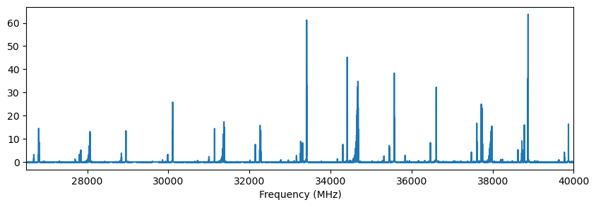
The CP-FTMW data for an experiment are stored in a BCFTMW object which is accessible as BCExperiment.ftmw. This object can be used to view data about the available FIDs and load them from disk. For a single FID acquisition like this, the FID is loaded with BCFTMW.get_fid(), which returns a BCFid object. The BCFID.ft() method computes the Fourier transform of that FID. As a quick example:

x,y = exp.ftmw.get_fid().ft()

fig,ax = plt.subplots(figsize=(10,3))
ax.plot(x,y)
ax.set_xlabel('Frequency (MHz)')
ax.set_xlim(26500,40000)

(26500.0, 40000.0)

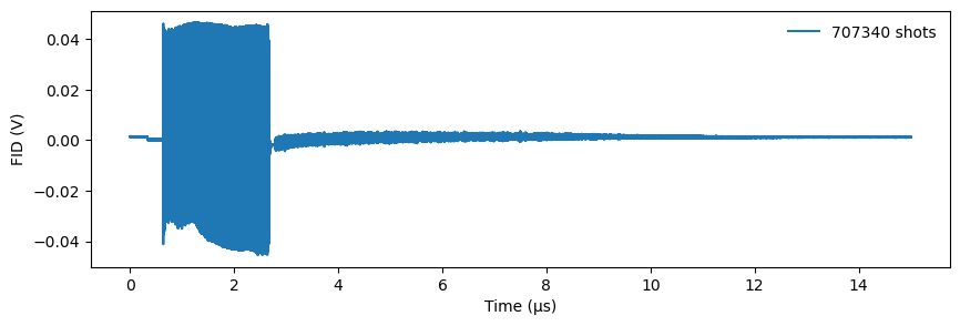
Taking a step back, the FID itself can be stored and visualized. The FID itself has BCFid.y() and BCFid.xy() methods which return arrays containing the FID data in units of V, and in the latter case, also the time array in units of s. For this FID, the chirp takes place from roughly 0.75 - 3.75 μs.

fid = exp.ftmw.get_fid()

fidx, fidy = fid.xy()
fig,ax = plt.subplots(figsize=(10,3))
ax.plot(fidx*1e6,fidy,label=f'{int(fid.shots)} shots')
ax.set_xlabel('Time (μs)')
ax.set_ylabel('FID (V)')
ax.legend(frameon=False)

<matplotlib.legend.Legend at 0x7f556485d1c0>

At this point it is important to note that fidy is a 2D numpy array. The second axis corresponds to the frame number. In this acquisition, there is only 1 frame, but for an acquisition configured with multiple records this number may be larger. A single frame can then be selected by slicing (e.g., fidy[:,3]).

fidy.shape

(750000, 1)

The contents of the fidparams.csv file are available as an attribute of the BCFTMW object.

exp.ftmw.fidparams

	spacing	probefreq	vmult	shots	sideband	size
index
0	2.000000e-11	40960	0.000002	707340	LowerSideband	750000
1	2.000000e-11	40960	0.000002	89820	LowerSideband	750000
2	2.000000e-11	40960	0.000002	179840	LowerSideband	750000
3	2.000000e-11	40960	0.000002	269840	LowerSideband	750000
4	2.000000e-11	40960	0.000002	359860	LowerSideband	750000
5	2.000000e-11	40960	0.000002	449860	LowerSideband	750000
6	2.000000e-11	40960	0.000002	539860	LowerSideband	750000
7	2.000000e-11	40960	0.000002	629860	LowerSideband	750000

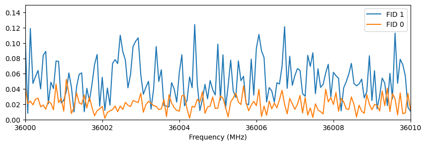
This experiment contains 2 FIDs: FID 0 is the final set of data and FID 1 was a backup that was taken 15 minutes into the acquisition. The BCFTMW.get_fid() function takes an optional argument that specifies the FID number to retrieve. We can therefore access the backup version with get_fid(1). The code below loads the backup and plots its FT together with the total, showing the decrease in noise level with increasing shots.

x2,y2 = exp.ftmw.get_fid(1).ft()
fig,ax = plt.subplots(figsize=(10,3))
ax.plot(x2,y2,label='FID 1')
ax.plot(x,y,label='FID 0')
ax.set_xlabel('Frequency (MHz)')
ax.set_xlim(36000,36010)
ax.set_ylim(0,0.15)
ax.legend()

<matplotlib.legend.Legend at 0x7f5562d4b580>

The BCFid.ft() function also allows for customizing the FID processing options like those in the Blackchirp program itself. The default values are read in from processing.csv, which is converted into a python dictionary named proc which is an attribute of BCFTMW. One notable difference in behavior: in the python module, points within “AutoscaleMHz” of the probe frequency are set to 0 to accommodate automatic autoscaling of the plot, while in Blackchirp itself those points are still shown but are not included when computing the vertical range of the FT.

exp.ftmw.proc

{'AutoscaleIgnoreMHz': '250',
 'FidEndUs': '15',
 'FidExpfUs': '0',
 'FidRemoveDC': 'false',
 'FidStartUs': '3.35',
 'FidWindowFunction': 'None',
 'FidZeroPadFactor': '0',
 'FtUnits': '6'}

The BCFid.ft() function allows for any of these settings to be overridden.

fid.ft?

Signature:
fid.ft(
    *,
    start_us: 'float' = None,
    end_us: 'float' = None,
    winf: 'str' = None,
    zpf: 'int' = None,
    rdc: 'bool' = None,
    expf_us: 'float' = None,
    autoscale_MHz: 'float' = None,
    units_power: 'int' = None,
    frame: 'int' = None,
) -> 'tuple[np.ndarray, np.ndarray]'
Docstring:
Compute the Fourier transform of the FID

By default, this computes the FT for each frame in the FID using the settings
stored in the proc dictionary. This behavior can be overridden by specifying
any combination of the keyword arguments.

Args:
    start_us: Starting time, in μs. Points at earlier times are set to 0.
    end_us: Ending time, in μs. Points at later times are set to 0.
    winf: Window function applied to points between start and end.
        This is passed directly to `scipy.signal.get_window <https://docs.scipy.org/doc/scipy/reference/generated/scipy.signal.get_window.html>`_.
    zpf: Zero-padding factor (positive integer). If nonzero, the FID is
        padded with zeroes until its length reaches the next power of 2,
        Then, its length is further extended by 2\*\*zpf.
    rdc: If true, the average of the FID is subtracted before the FT is
        computed.
    expf_us: Time constant for an exponential decay filter, in μs.
    autoscale_MHz: Range of FT points to set to 0, relative to the Downconversion
        LO frequency. Useful for suppressing noise near DC.
    units_power: FT is scaled by 10\*\*units_power. For μV units, set
        units_power=6.
    frame: Apply FT to only the specified frame.

Returns:
    Frequency array (MHz), Intensity array

Raises:
    ValueError: If supplied arguments are invalid

Examples:
    Assuming a BCFid object named ``fid``::

        #default FT calculation
        x,y = fid.ft()

        #override some processing settings
        x,y = fid.ft(start_us=3.0,rdc=False,units_power=3)

        #compute ft for only frame 3 (assuming the number of frames is >=4)
        x,y = fid.ft(frame=3)

        #average all frames, then apply a custom window function
        fid.average_frames()
        p = 1.5
        sigma = len(fid)//5
        x,y = fid.ft(winf=('general_gaussian',p,sigma))
File:      ~/github/blackchirp/src/python/blackchirp/src/blackchirp/bcfid.py
Type:      method

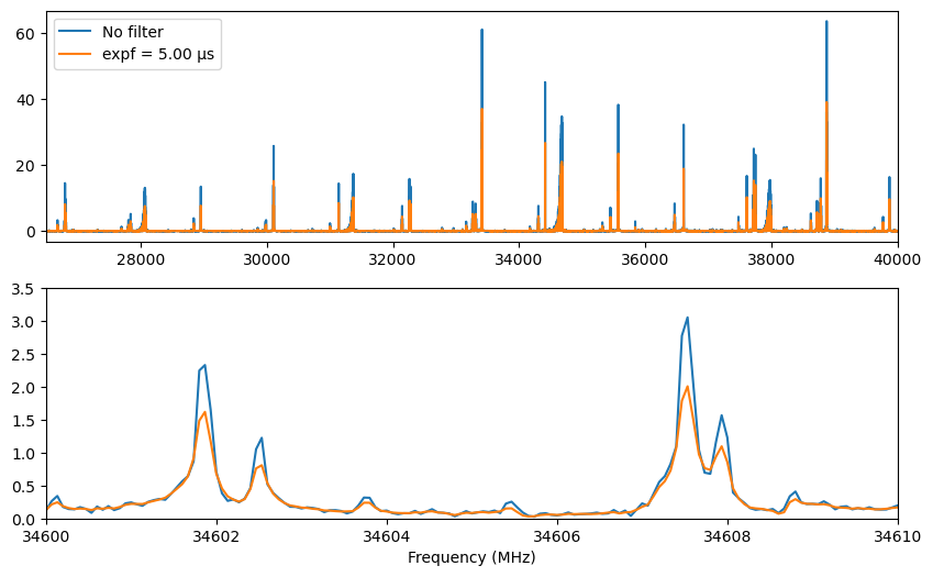
For example, to apply an exponential filter and compare with the original data:

expf = 5.0
x3,y3 = exp.ftmw.get_fid().ft(expf_us=expf)

fig,axes = plt.subplots(2,1,figsize=(10,6))
for ax in axes:
    ax.plot(x,y,label='No filter')
    ax.plot(x3,y3,label=f'expf = {expf:.2f} μs')
axes[0].set_xlim(26500,40000)
axes[1].set_xlim(34600,34610)
axes[1].set_ylim(0,3.5)
axes[0].legend()
axes[1].set_xlabel('Frequency (MHz)')

Text(0.5, 0, 'Frequency (MHz)')

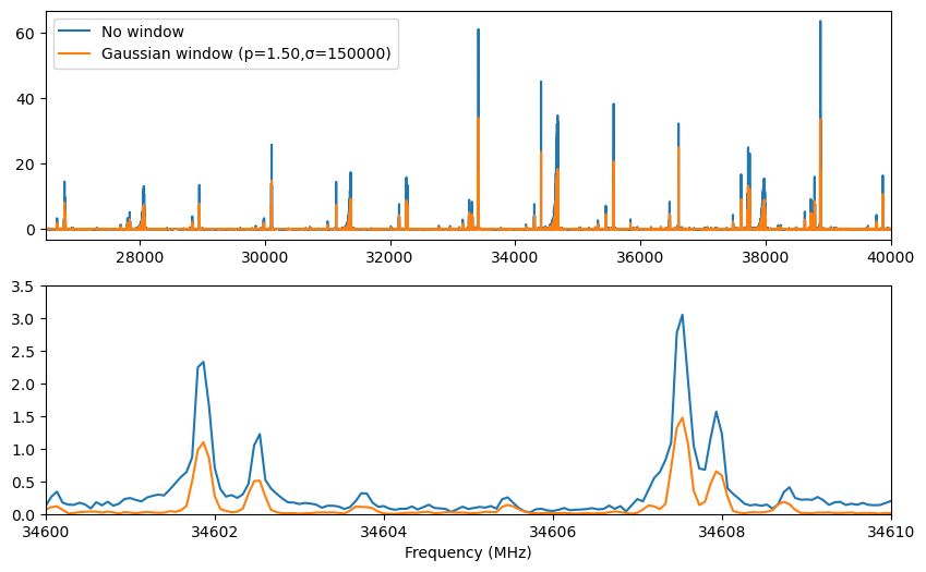
A greater variety of window functions is available in the Python module compared with Blackchirp. The winf parameter can be set to any value supported by scipy.signal.get_window. For example, a generalized Gaussian window with variable p and σ parameters can be used by passing a tuple with the window name and parameter values:

p = 1.5
sigma = len(fid)//5
x4,y4 = fid.ft(winf=('general_gaussian',p,sigma))

fig,axes = plt.subplots(2,1,figsize=(10,6))
for ax in axes:
    ax.plot(x,y,label='No window')
    ax.plot(x4,y4,label=f'Gaussian window (p={p:.2f},σ={int(sigma)})')
axes[0].set_xlim(26500,40000)
axes[1].set_xlim(34600,34610)
axes[1].set_ylim(0,3.5)
axes[0].legend()
axes[1].set_xlabel('Frequency (MHz)')

Text(0.5, 0, 'Frequency (MHz)')

Like the FID, the FT y array is 2-dimensional, where the second axis corresponds to the frame number. By default, the FT is applied to all frames at once; if only a single frame is desired, pass its index as the frame parameter.

y.shape

(375001, 1)