Viewing LIF Data

The LIF tab provides real-time and post-acquisition visualization of LIF data. It is visible in the main window whenever the LIF module is enabled (see Application Configuration).

Layout

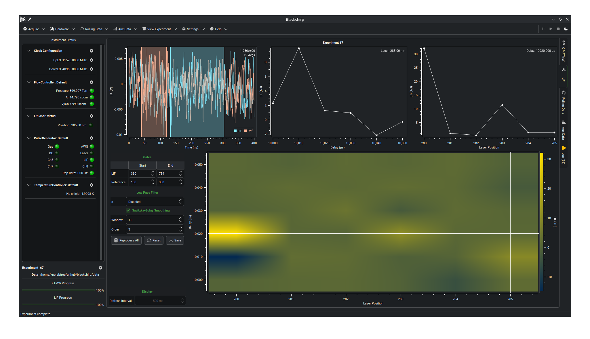
A bold header at the top names the loaded experiment and links to its data folder. Below the header are two rows: an upper row of three plots side by side, and a lower row holding the processing panel on the left and the 2D spectrogram on the right.

Time trace (upper row, left)

Displays the digitizer waveform for the scan point selected on the 2D spectrogram. During an acquisition it updates at the rate set by the refresh interval control, showing the accumulated average waveform at the current scan position. Shaded regions mark the LIF and reference integration gates. The LIF waveform and, when the reference channel is enabled, the reference waveform are drawn on the same plot and distinguished by an in-canvas legend in the lower-right corner.

Delay slice (upper row, center)

Plots integrated LIF signal as a function of delay time, evaluated at the laser-frequency column currently selected on the 2D spectrogram.

Laser slice (upper row, right)

Plots integrated LIF signal as a function of laser position, evaluated at the delay row currently selected on the 2D spectrogram.

2D spectrogram (lower right)

Renders the full two-dimensional dataset as a false-color map with delay on one axis and laser frequency on the other. Each cell represents one scan point; its color encodes the integrated LIF signal at that point. The color scale updates automatically as new data arrive.

Selecting a scan point on the 2D spectrogram

The 2D spectrogram carries two cursors — a horizontal line at the selected delay and a vertical line at the selected laser position — that drive both slice plots and the time trace. The selected point can be moved in two ways:

• Drag a cursor. Click and drag the horizontal cursor to change the delay selection (updating the laser slice and the time trace), or the vertical cursor to change the laser-frequency selection (updating the delay slice and the time trace).

• Right-click for the context menu. Right-click anywhere on the spectrogram and choose Move delay cursor here, Move frequency cursor here, or Move both cursors here to jump the corresponding cursor(s) to the click location. The same menu has a Follow live data entry that re-locks both cursors to the most recent live acquisition point.

Dragging a cursor or invoking either of the move actions detaches the display from live-following; choose Follow live data to re-attach.

Processing panel

The processing panel occupies the lower-left of the tab. It exposes the integration gate positions, optional smoothing filters, and the post-acquisition workflow buttons, grouped under the Gates, Low Pass Filter, and Savitzky-Golay Smoothing section headings.

The panel is disabled during an acquisition: while data is being collected, the live plots integrate using the gate and filter values from the LIF Configuration. The panel becomes editable once the acquisition completes. After that, changing any value redraws the time trace and its shaded gates immediately, but the integrated values on the slice plots and the 2D spectrogram are recomputed only when Reprocess All is pressed.

Gates

A table with LIF and Reference rows and Start and End columns. Each cell is a sample-point index into the running accumulated waveform; the gate it defines is applied before the integrated value is computed. Hold Ctrl while scrolling a value to adjust in steps of 10. The Reference row is editable only when the reference channel is enabled in the LIF Configuration. See LIF Configuration for the relationship between sample points and time.

Low Pass Filter

The α value applies a single-pole IIR low-pass filter to each waveform before integration:

\[x_n = \alpha \, x_{n-1} + (1 - \alpha) \, x_n\]

Setting α to 0 (the special value displayed as Disabled) bypasses the filter. Higher values increase smoothing at the cost of temporal resolution within the waveform.

Savitzky-Golay Smoothing

A checkable section. When enabled, a Savitzky-Golay polynomial smoothing filter is applied to each waveform before integration, and two settings appear: Window (the filter window size; forced to an odd number and at least 3) and Order (the polynomial order; at least 2 and strictly less than the window size). When the section is unchecked, the two settings are hidden.

The three buttons at the bottom of the processing panel operate on the stored data and on processing.csv. They are enabled only after the acquisition completes:

• Reprocess All — re-integrates every stored waveform using the current gate and filter settings, then redraws all plots.

• Reset — restores the gate and filter settings to the values most recently saved to processing.csv.

• Save — writes the current gate and filter settings to lif/processing.csv in the experiment folder. These become the default values applied when the experiment is opened in the future.

Note

The recorded time-trace data on disk are never modified. Each scan point’s averaged waveform is written during acquisition and remains untouched thereafter; Save only updates processing.csv with the new default gate and filter values for that experiment. Reprocess All likewise re-integrates the stored waveforms in memory and updates the plots, without rewriting the trace files.

Refresh interval

Below the processing panel, a Display section holds the Refresh Interval spin box, which sets how frequently the plots are updated during an acquisition, in milliseconds. It is active only while data is being collected. Shorter intervals give a more responsive display at the cost of additional processing overhead. The plots are also redrawn whenever a processing setting changes. Multiple refresh requests that arrive while a previous update is still being processed are coalesced; only the most recent request is acted upon.