Viewing FTMW Data
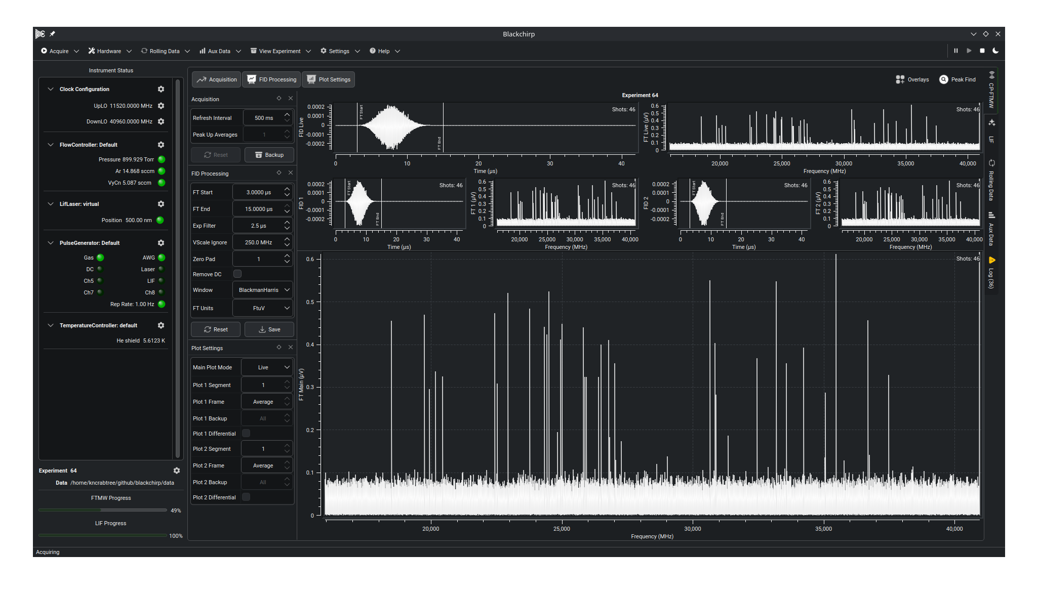
The CP-FTMW tab visualizes and processes FID and Fourier-transform data, both during an acquisition and when reviewing a completed experiment. During an acquisition, seven plots are shown. The uppermost pair, FID Live and FT Live, always display the most current data and are removed when the acquisition completes. The pairs FID 1/FT 1 and FID 2/FT 2 display user-selectable views of the data (see Plot Settings). Most interaction takes place on the large Main FT plot, which by default follows the live data during an acquisition and switches to the FT 1 view when the experiment ends. Zooming, panning, peak finding, and other plot interactions are available both during and after an acquisition; see the Plot Controls page for details. The bold header above the plots names the loaded experiment and, except in Peak-Up mode, links to that experiment’s data folder.
The toolbar across the top toggles a set of dockable side panels. Acquisition, FID Processing, and Plot Settings open on the left; Overlays and Peak Find open on the right. Each panel is a separate dock that can be resized, dragged to either side, tabbed with another panel, floated into its own window, or closed; clicking its toolbar button again hides it. The panels are described in the sections below.
Plot processing is queued and runs on a separate thread from the real-time averaging, so during a fast acquisition the displayed data lag the accumulated data slightly. Plots also refresh whenever a setting that affects them changes. If several refresh requests arrive while an FT is being computed, Blackchirp keeps only the most recent.
Acquisition
The Acquisition panel collects the controls that apply while data is being collected. It is not present in the Blackchirp Viewer, where no acquisition is in progress.
Refresh Interval: How often the live FID and FT plots are redrawn during an acquisition.Peak Up Averages: The number of shots in the rolling average shown on the live plots. Enabled only in Peak-Up mode, where it can be changed on the fly. The adjacentResetbutton discards the current rolling-average accumulation and restarts it.Backup: Writes a snapshot of the current FID list to disk on demand (see Manual Backup).
Manual Backup
The Backup button in the Acquisition panel (archive-box icon) writes a snapshot of the current FID list to disk on demand. It is enabled during a live acquisition in the single-segment, backup-capable modes — Target Shots, Target Duration, and Forever — and is disabled for Peak Up, LO Scan, and DR Scan, which either do not produce on-disk backups (Peak Up) or write a backup automatically at each segment boundary (LO Scan and DR Scan). Because the Acquisition panel is absent in the Experiment Viewer, the button is unavailable there as well.
The manual backup uses the same on-disk format and numbering as periodic backups configured via the Backup Interval setting in Common Settings — backups are saved as 1.csv, 2.csv, etc. in the experiment’s fid directory, with the final FID list saved as 0.csv when the experiment ends. Once written, a manual backup is selectable from the Backup row on the Plot Settings panel, and Differential mode shows the data accumulated since that checkpoint.
When the button is clicked the status bar briefly displays Manual backup requested. When the write completes — typically within a fraction of a second — the status bar updates to Manual backup complete (backup N) and a corresponding Highlight-level entry is added to the log so the backup number can be recalled later. After the status-bar message expires, the bar reverts to Acquiring or Paused as appropriate.
If a periodic backup is already in flight when the button is clicked, the request is folded into the in-flight write rather than queued — the periodic backup is the same snapshot the manual request would produce, so it is simply relabeled in the completion message.
FID Processing Settings
The FID Processing panel holds the settings that control how each FID is transformed before it is displayed. They apply to the data shown on every plot:
FT Start: The starting time for the data to be Fourier transformed. Points before this time are zeroed out. This setting is useful when the digitizer is triggered prior to the excitation chirp. In this case, FT Start can be set to 0 to view the chirp and monitor phase coherence. FT Start can also be adjusted to exclude signals from ringing of the excitation pulse or switch bounce.FT End: The ending time for the FT. Points after this time are zeroed out. Useful in conjunction with FT Start to assess the T2 relaxation time of the FID.Exp Filter: Time constant for an exponential filter applied to the FID prior to the FT. Matching the filter time constant to the natural T2 relaxation time provides noise suppression.VScale Ignore: A frequency range near the LO to ignore when computing the autoscale range. CP-FTMW data often have large uninteresting signals near DC, and this setting prevents those from overwhelming the default vertical scale.Zero Pad: Appends zeros to the FID to artificially increase the digital resolution of the FT. A setting of 1 appends zeros until the length of the array is double the next power of two. For example, for a record length of 750,000 points, the next power of two is 2^20, or 1,048,576 points. With Zero Pad = 1, zeros are appended until the data length is 2^21, or 2,097,152 points. Each subsequent increase of the Zero Pad setting increases the length by another factor of 2.Remove DC: Subtracts the average value of the FID prior to the Fourier transform. Removes large-envelope DC artifacts.Window: Applies a window function prior to Fourier transformation. Window functions suppress spectral leakage from strong signals, which tends to obscure nearby weaker transitions. A window cuts down on these sidelobes at the expense of reducing the signal-to-noise ratio slightly and decreasing the spectral resolution. See the CP-FTMW Data page for the definitions of the window functions implemented in Blackchirp.FT Units: Changes the vertical scaling of the FT.Reset: Restores processing settings to the most recently saved values.Save: Writes the current processing settings to aprocessing.csvfile. Processing settings are written when an experiment first starts and may be overwritten at any time.
The FID plots show the post-processed FID; the FT plots show its Fourier transform.
Plot Settings
The Plot Settings panel controls what data each plot displays.
Main Plot Mode selects the source for the large Main FT plot:
Live: The Main plot shows the live data. For acquisition modes that change the clock settings (LO Scan, DR Scan), it follows the acquisition settings as they change. At the end of an acquisition this option is disabled and the mode changes toFT1ifLivewas selected.FT1: The Main plot mirrors theFT 1plot, including its segment, frame, and backup selections.FT2: The Main plot mirrors theFT 2plot, including its segment, frame, and backup selections.FT1_minus_FT2: The Main plot shows the result of subtractingFT 2fromFT 1.FT2_minus_FT1: The Main plot shows the result of subtractingFT 1fromFT 2.Upper_SideBand: Available only in LO Scan mode. Performs sideband deconvolution using only the higher-frequency sideband.Lower_SideBand: Available only in LO Scan mode. Performs sideband deconvolution using only the lower-frequency sideband.Both_SideBands: Available only in LO Scan mode. Performs sideband deconvolution using both sidebands.
Below the mode selector, the Plot 1 and Plot 2 rows independently choose what the FT 1 and FT 2 plots show:
Segment: For acquisition modes that involve multiple hardware settings in a single experiment (e.g., LO Scan, DR Scan), each individual hardware setting is associated with a “Segment.” The nomenclature comes from segmented CP-FTMW spectroscopy, which is implemented as an LO Scan in Blackchirp. Changing the segment shows the data associated with each individual LO tuning in such a scan.Frame: For “Multiple Record” acquisitions (see the Digitizer Setup page for more detail), this controls which individual record is displayed, indexed starting from 1. The special valueAverageco-averages the individual records.Backup: For long acquisitions in which backups are enabled, this selects the FID and FT associated with each backup checkpoint.Differential: If checked, the selected backup is subtracted from the current FID, allowing recent signal levels to be viewed during long integrations.
In LO Scan mode the panel also shows the sideband-deconvolution controls — SB Frame, SB Min Offset, SB Max Offset, SB Avg Algorithm, and a Reprocess Sidebands button. Their meaning is described in Sideband Deconvolution below.
Overlays
The toolbar’s Overlays button (squares-plus icon) shows the Overlay Manager panel. Overlays superimpose additional data on the FT plots for comparison and analysis. For detailed information on creating and managing overlays, see Overlays.
Note
Overlay settings are saved with the experiment and restored when the experiment is reopened.
Curve Autoscale
Each curve displayed on the FT plots has an Autoscale attribute that controls whether that curve participates in the vertical autoscale computation. By default, all curves are included. To toggle the autoscale participation of an individual curve, right-click on the plot to open the context menu, expand the Curves submenu, select the curve of interest, and check or uncheck the Autoscale checkbox in the curve’s appearance panel.
Disabling autoscale for a curve causes the vertical scale to be computed from the remaining autoscale-enabled curves only. This is useful when one curve (for example, an overlay) has a much larger amplitude than the primary FT data and would otherwise compress the vertical range.
Peak Find
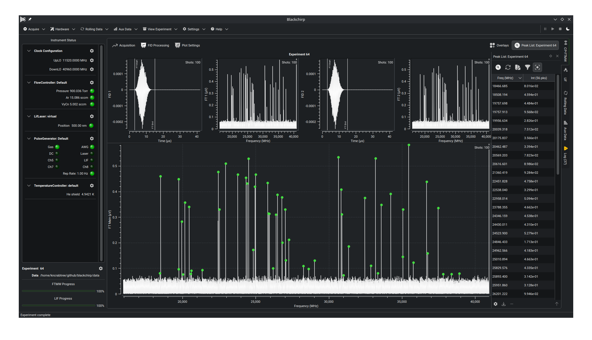
The Peak Find panel runs a rough peak-finding algorithm over the current FT and lists the detected peaks. The FT is passed through a Savitzky-Golay filter that returns the second derivative of a smoothed copy of the spectrum, determined by a window size (which must be odd) and a polynomial order used to fit the points within the window (which must be less than the window size). A peak is reported where the second derivative has a five-point local minimum and the corresponding point in the FT exceeds an estimate of the local noise level by at least the configured SNR.
Detected peaks are marked on the FT plots and listed in the panel’s table by frequency and intensity. The panel’s toolbar provides:
Find Now: Runs the search once on the current FT.Live Update: Re-runs the search automatically whenever the FT changes.Appearance: Edits the peak-marker appearance.Filter: Shows a display-filter grid that hides listed peaks outside a frequency or intensity range. The filter affects only what the table and markers show; it does not change the search.In view: Restricts the list to peaks within the Main FT plot’s currently visible frequency range.
A second row of actions manages the list:
Options...: Opens the Peak Finding Options dialog (frequency range, SNR, window size, polynomial order, and the navigation-window half-width).Export...: Exports the list (see below).Remove: Removes the selected peaks from the list.Show Parent: Raises the FTMW view; shown when the panel is floating.
The list also drives plot navigation. Acting on a peak frames it on a plot, centering the view on the peak’s frequency with a window whose half-width is set by Navigation Half-Width in the Peak Finding Options dialog:
Double-clicking a row centers the Main FT plot on that peak.
Right-clicking a row opens a context menu with
Center main plotand aCenter onsubmenu that lists every plot (Main,FT 1,FT 2) so a specific plot can be centered instead.The arrow keys navigate from the keyboard, with the Main FT plot re-centering on each step.
UpandDownmove one row at a time through the list as displayed, following the current sort and display filter.LeftandRightinstead step to the next lower- or higher-frequency peak in the full list, regardless of how the table is sorted or filtered; with no peak yet selected,Leftjumps to the lowest-frequency peak andRightto the highest.Enterre-centers on the current peak.
The search parameters are remembered per experiment. Each experiment stores its own values in a peakfind.csv file; an experiment with no saved file uses the application-wide defaults, which are updated whenever the options are changed.
Note
This peak-finding algorithm works reasonably well for windowed data, but often finds many false positives in the absence of a window function in the vicinity of strong signals with significant spectral leakage.
Export... writes the peak list to a CSV file or to an FTB file, the latter of which is an input for the cavity FTMW software QtFTM.
Sideband Deconvolution
The sideband deconvolution algorithm employed by Blackchirp is designed to suppress image frequencies in an LO scan. Most segmented LO scanning spectrometers employ a low-frequency chirp which is mixed up to the target frequency via a tunable LO. This leads to two simultaneous chirps: one at the LO frequency + chirp frequency and the other at the LO frequency - chirp frequency. If both of these are within the bandwidth of the amplifier, then the sample experiences both chirps simultaneously, yielding molecular FID signals in both windows. However, upon downconversion with a second mixer, both of these sidebands are downconverted to the same range of frequencies, so each downconverted frequency in the FT may correspond to either of the two sidebands. This uncertainty is eliminated by tuning the LO frequency slightly and observing which “direction” the signal moves relative to the LO.
In Blackchirp, the sideband deconvolution algorithms are based on overlapping frequency-shifted versions of the FT onto a common frequency grid. Because the spectra are acquired at different LO tunings, the frequency bins for each FT may not perfectly align. Blackchirp computes a global frequency grid spanning all sidebands and uses linear interpolation to resample all FTs onto that grid.
Consider the simple case of an LO frequency of 10 GHz and a signal observed at 500 MHz in the FT (with a digitizer and chirp bandwidth of 1 GHz). This may correspond to a molecular frequency of either 9.5 or 10.5 GHz. Next, increase the LO frequency by 100 MHz to 10.1 GHz. If the molecular frequency is 10.5 GHz, the new frequency observed by the digitizer is 400 MHz, while if it is 9.5 GHz, then the new digitizer frequency is 600 MHz. In the “Upper Sideband” deconvolution algorithm, it is assumed that all molecular emission occurs in the higher-frequency sideband. In this case, Blackchirp would compute 2 FTs for the two LO tunings: one spanning 10-11 GHz, and the other spanning 10.1-11.1 GHz. Blackchirp aligns these two tunings and co-averages the spectra where they overlap. In both cases, the signal appears at an apparent frequency of 10.5 GHz, so the signal adds.
However, in the “Lower Sideband” algorithm, Blackchirp would assign the frequency axes as 10.0-0.0 and 10.1-9.1 GHz, respectively. Because the true molecular frequency was 10.5 GHz, the signal which appeared at a 9.5 GHz apparent frequency appears with an apparent frequency of 9.7 GHz (10.1 GHz - 0.4 GHz) in the second LO tuning. Co-averaging these two spectra attenuates the signal.
In “Both Sidebands” mode, both sideband deconvolutions are computed and a composite spectrum is created by concatenating their respective frequency axes. This mode has the additional benefit of providing additional averages when the same frequency is covered in both sidebands as the LO is tuned over a broad range.
Warning
If the effective sensitivity of the two sidebands is very different (which could be caused by variable mixer efficiency or by choosing LO tunings too close to the limits of the amplifier bandwidth), then “Both Sidebands” mode could result in artificial signal suppression.
The sideband controls in the Plot Settings panel — shown only in LO Scan mode — tune the deconvolution. After changing any of them, click Reprocess Sidebands to re-run the deconvolution with the current settings.
SB Frame: If multiple FIDs are acquired per pulse, this selects which frame is used. The special valueAverageaverages all frames.SB Min Offset: Minimum offset frequency (relative to the LO frequency) of the FT to include when processing each sideband. By default this should be set to the minimum chirp frequency relative to the LO. Blackchirp calculates this value automatically from the Rf Configuration and Chirp Configuration.SB Max Offset: Maximum offset frequency (relative to the LO frequency) of the FT to include when processing each sideband.SB Avg Algorithm: The co-averaging algorithm used when overlapping the frequency-shifted spectra. Blackchirp does not calculate the arithmetic mean of the spectra; this would provide very poor image suppression. The available options are:Harmonic Mean: A shots-weighted harmonic mean, a measure of central tendency strongly biased toward the lowest value in the set. This is desirable for sideband suppression, as the spectrum should average strongly toward 0 if a line is present in only one of the shifted spectra. For this reason it is the default. Let s1 and s2 be the numbers of shots for the two data points y1 and y2, respectively. Assuming all samples and shots are positive and nonzero, the weighted harmonic mean is:
\[y_{\text{avg}} = \frac{s_1 + s_2}{\frac{s_1}{y_1} + \frac{s_2}{y_2}}\]Geometric Mean: A shots-weighted geometric mean, which falls between the harmonic and arithmetic means. The weighted geometric mean is:
\[y_{\text{avg}} = \exp\left(\frac{s_1\ln y_1 + s_2\ln y_2}{s_1 + s_2}\right)\]