Plot Controls
All plots in Blackchirp share a common set of zoom/pan controls and customization options. Each plot is configured individually, and the most recent settings are recalled when the program starts. The appearance of each curve, the vertical axis a curve is plotted against, the plot grid, and reusable curve presets are all configurable per plot.
Zooming and Panning
Zooming is performed with the mouse wheel or by left-clicking and
dragging a rectangle on the plot.
While dragging a rectangle, press the z key to cancel.
With the mouse wheel, scrolling up zooms in and scrolling down zooms
out.
Rectangle dragging only zooms in; use the mouse wheel or keyboard to
zoom out.
By default, zooming affects the X axis and both Y axes simultaneously.
This behavior can be changed using modifier keys:
Ctrl: Zoom X axis only; Y axes are fixed.Shift: Zoom both Y axes, keeping X axis fixed.Meta(Windows key): Zoom left axis only (only for scroll zooming).Alt: Zoom right axis only (only for scroll zooming).
To zoom out immediately to the full range of the data, double-click the
plot or press the Home key.
Alternatively, right-click the plot and choose Autoscale.
The zoom limits are determined by the X and Y range spanned by the data.
Panning is performed by middle-clicking anywhere on the plot and dragging. As with zooming, panning is limited to the range of the data displayed on the plot, so it has no effect when the plot is at full scale.
Keyboard controls are also available for zooming and panning:
Arrow keys: Step the plot in the direction pressed by 50% of the scale width.
Alt+ Arrow keys: Step the plot in the direction pressed by 10% of the scale width.Shift+Up/Down: Zoom in/out vertically by 10%. By default, the zoom is symmetric about 0.0 (but see theY Center?setting below).Ctrl+Up/Down: Zoom in/out vertically by 50%. By default, the zoom is symmetric about 0.0.Shift+Right/Left: Zoom in/out horizontally by 10%. The zoom is symmetric about the center of the plot.Ctrl+Right/Left: Zoom in/out horizontally by 50%. The zoom is symmetric about the center of the plot.
Plot Configuration Options
The right-click context menu contains options that control the appearance and behavior of the plot as a whole:
Autoscale: Reset both axes to show the full range of the data.Zoom Settings:Y Center?: Toggles whether zooming with theUp/Downarrows is symmetric about the plot center (checked) or about 0.0 (unchecked).Wheel Zoom Factors: Sets the zoom speed for each axis when scrolling the mouse wheel. Larger numbers zoom by a greater factor per wheel step. The default value for each axis is 0.1.
Tracker: Enable the tracker to display the coordinates of the mouse cursor on the plot. For each axis, you can configure the number of decimals displayed and, optionally, switch to scientific notation.Grid: Configure the appearance of major and minor gridlines. The line style and color are configurable independently for each type of gridline.Curves: Per-curve appearance and preset controls; see Curve Configuration Options below.
On the Rolling and Aux Data plots, two extra entries appear at the bottom of the menu:
Push X Axis: Set the X scale of all other plots to match the selected plot.Autoscale All: Apply the autoscale action to all plots.
Curve Configuration Options
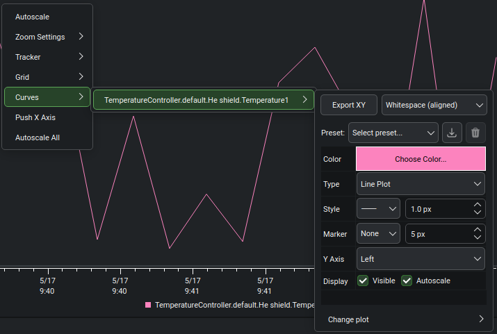
The Curves entry in the context menu opens a submenu listing every
curve on the plot. Selecting a curve opens its submenu, which contains,
top to bottom: an Export XY row, the curve appearance panel (a
preset bar above an appearance table), and — on the Rolling and Aux
Data plots only — a Change plot submenu. Changes made in the
appearance panel are applied to the curve immediately.
Export XY: Writes the data currently displayed for this curve to a text file. The drop-down beside the button selects the column delimiter, applied to every subsequent export and remembered application-wide (shared between Blackchirp and the viewer):Semicolon,Comma,Tab, orWhitespace (aligned)— the last left-justifies the columns for easy reading without any leading whitespace, so it still loads with a whitespace separator (e.g. pandassep=r"\s+").
The preset bar carries a Preset drop-down and save/delete buttons;
it is described under Curve Presets below. The appearance table has
one row per setting:
Color: Opens a color picker for the curve color.Type: How the curve is rendered —Line Plot,Stick Plot,Step Plot,Scatter Dots, orNo Curve.Style: The line style (solid, dashed, dotted, etc.;Nonesuppresses the line) and, beside it, the line width in pixels.Marker: The symbol drawn at each data point (Nonesuppresses markers) and, beside it, the marker size in pixels.Y Axis: Which Y axis the curve is plotted against (LeftorRight).Display: Two checkboxes —Visible(whether the curve is drawn) andAutoscale(whether the curve is included when the axis limits are computed during an autoscale operation).
On the Rolling and Aux Data plots, the Change plot submenu moves
the curve to a different plot in the grid. The plots are numbered from
left to right, then top to bottom.
Curve Presets
The preset bar at the top of the curve appearance panel saves a full set of appearance settings — color, type, width, line style, marker, marker size, visibility, autoscale flag, and Y axis assignment — under a name and applies that combination to any curve in any plot. Presets are stored globally; they are shared across plots and persist across program runs.
Default Presets
Blackchirp ships with nine default presets that are created the first time the program is run:
Curve - Primary,Curve - Secondary,Curve - Tertiary— solid line plots in three palette-derived colors.Stem - Primary,Stem - Secondary,Stem - Tertiary— stick (stem) plots in the same three colors.Scatter - Circles,Scatter - Squares,Scatter - Diamonds— marker-only scatter plots with circular, square, and diamond markers.
Default presets cannot be deleted or renamed, but their contents can be
overwritten (see Saving a Preset below).
When a default preset is selected in the Preset drop-down, the
delete button is disabled.
Applying a Preset
To apply a preset to the current curve, choose its name from the
Preset drop-down.
The curve updates immediately, and the appearance table below reflects
the preset’s values.
Saving a Preset
The save button (disk icon) opens the Save Curve Appearance Preset dialog, which offers two modes:
Create new preset: Enter a name for a new preset. A suggestion derived from the current appearance settings is pre-filled and may be edited. If the chosen name matches an existing preset, a confirmation prompt appears before the existing preset is overwritten.
Overwrite existing preset: Choose an existing preset from the drop-down (default presets are tagged
(default)) and replace its contents with the current appearance. This is the only way to modify a default preset.
After saving, the new or updated preset is selected in the Preset
drop-down.
Deleting a Preset
To delete a custom preset, select it in the drop-down and click the delete button (trash icon). A confirmation dialog appears before the preset is removed. The delete button is disabled when no preset is selected or when the selected preset is a default.