Overlays
An overlay is an additional curve drawn on top of an FT plot for comparison with the experimental spectrum. Overlays compare two experiments side by side, display predicted line lists from spectroscopic fitting programs, and import arbitrary XY data from other sources. Overlays are saved with the experiment and restored automatically the next time it is opened; the on-disk format is described on the CP-FTMW Data page.
Overlay Manager
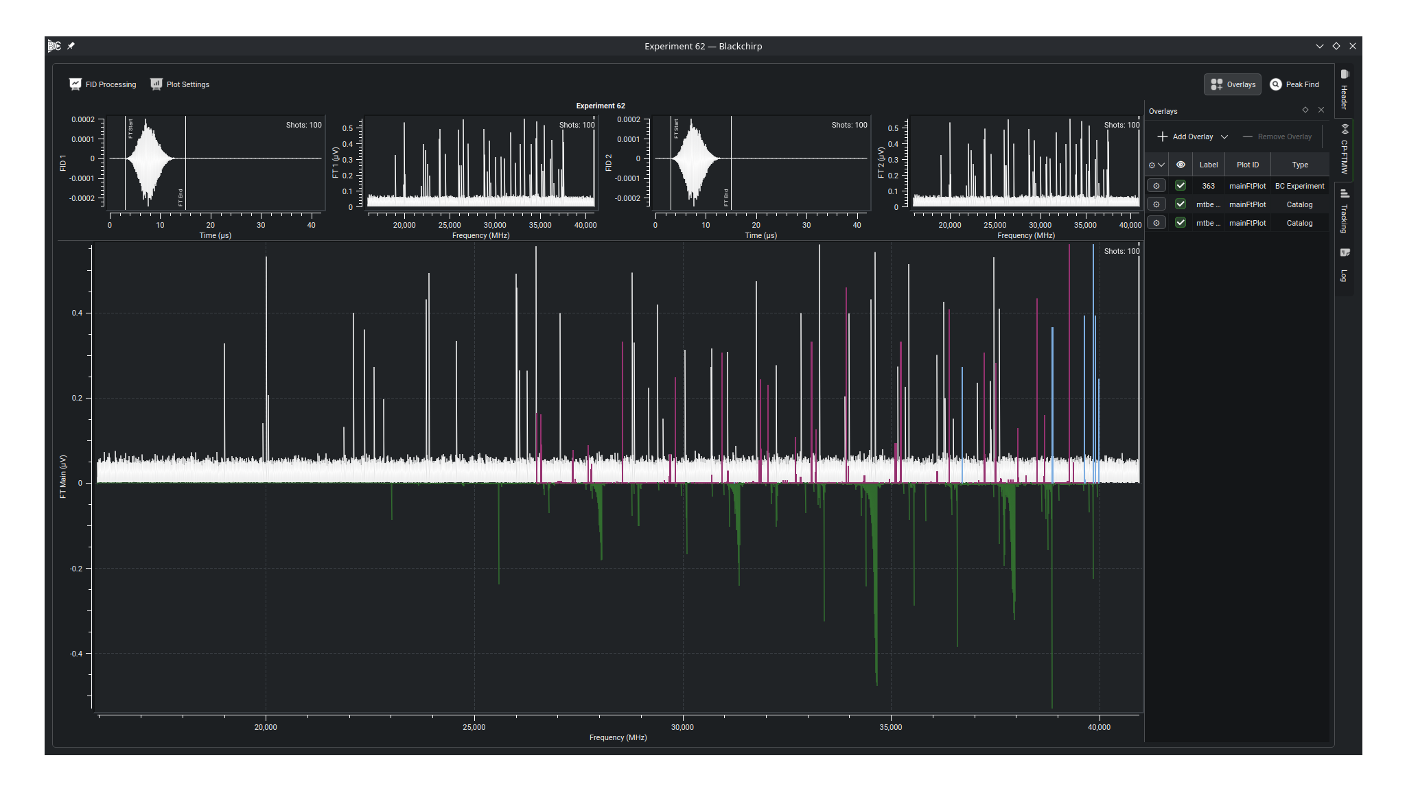
The Overlay Manager is opened from the Overlays button on the CP-FTMW toolbar; see Viewing FTMW Data for the toolbar context. It docks alongside the FT plots (shown open in the overview above) and lists every overlay defined for the experiment, one per row, with a toolbar of actions:
Add Overlay: Opens a menu of overlay types; choosing one opens the creation dialog for that type.Remove Overlay: Deletes the selected overlay(s).Show Parent: Raises the FTMW view the manager belongs to. This action appears only when the manager is floating (detached from the main window into its own top-level window).
Each row has the following columns:
Configure (gear icon): Opens the same dialog used during creation; changes apply on close.
Enabled (eye icon): Toggles the overlay’s visibility on the plot without deleting it.
Label: Editable name for the overlay, unique within the experiment. Special characters (including semicolons) are replaced with underscores when the label is written to disk.Plot ID: Which plot the overlay is drawn on. The same source can be added more than once to display on different plots.Type: Catalog, Generic XY, or BC Experiment.Comment: Free-form notes. May not contain semicolons.
Right-clicking a row offers Configure..., Edit Comment..., a Curve Appearance submenu, and copy/paste of the overlay’s data settings (Y scale, offset, frequency filtering) and its curve appearance (color, line style, thickness). Undo reverts the most recent paste. The copy/paste actions also have keyboard shortcuts:
Ctrl+C/Ctrl+V: Copy/paste curve appearance.Ctrl+Shift+C/Ctrl+Shift+V: Copy/paste data settings.Ctrl+Z: Undo the most recent paste.
Creating an Overlay
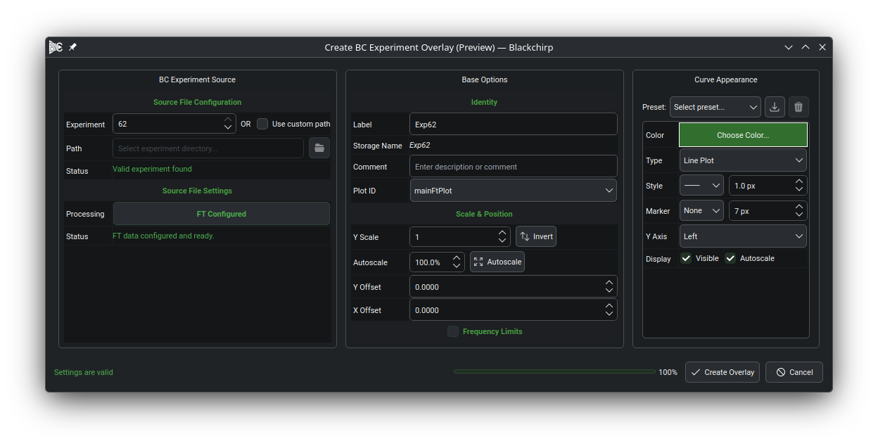
Click Add Overlay and choose a type from the menu. The creation dialog opens for that type, titled Create <Type> Overlay (Preview), with three panels: a type-specific source panel on the left (described under Overlay Types below), Base Options in the center, and Curve Appearance on the right. The plot shows a live preview as settings change. Click Create Overlay to add the overlay or Cancel to discard it.
Base Options holds settings common to every type: the label, comment, and target plot; the Y scale (with Invert and Autoscale); X and Y offsets; and an optional Frequency Limits group that restricts the drawn curve to a frequency window. Curve Appearance is the standard per-curve control described in Curve Configuration Options, including appearance presets.
The configuration in the source panel differs by overlay type, as described below. The same dialog is reused by the Configure action to edit an existing overlay.
Overlay Types
Blackchirp supports three overlay types, each backed by a different file format.
BC Experiment
Loads the FT data from another Blackchirp experiment, selected by experiment number or by browsing to a custom path. The experiment metadata (LO frequency, shot counts, FT processing settings) is preserved, and the FT can be reprocessed with the standard processing controls. This is the most direct way to compare two experiments acquired under different conditions (e.g., discharge on vs. off, or different sample backing pressures).
Catalog
Displays a stick spectrum or convolved lineshape from a spectroscopic fitting program. SPCAT and XIAM output formats are supported. Each transition retains its quantum numbers and source-program metadata, shown in the curve tooltip.
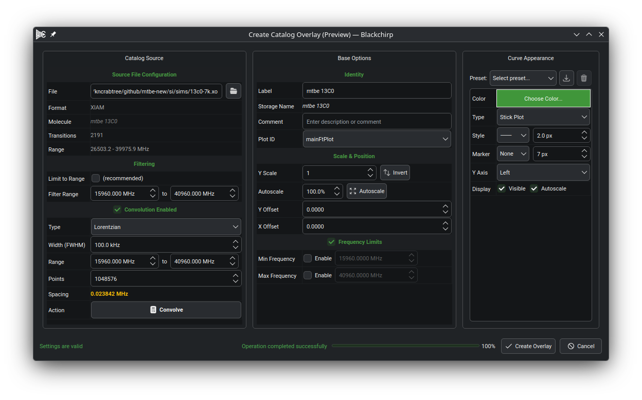
The Filtering section limits the overlay to a subset of the catalog by frequency. Restricting the range reduces both processing time and memory use; for very large catalogs (>100,000 transitions), pre-filtering the file to the relevant range is recommended.
Enabling Convolution Enabled convolves the stick spectrum with a Lorentzian or Gaussian lineshape of a user-defined FWHM for direct comparison with experimental data. Convolution runs on a background thread; for large catalogs it may take a minute or more, and progress is reported in a cancellable dialog. Results are cached, so repeating the same parameters returns immediately.
Generic XY
Loads arbitrary XY data from a delimited text file. Comma-, semicolon-, tab-, and space-separated formats are recognized, and a custom delimiter may be set manually. Auto-Detect Format infers the delimiter and header line count; the X and Y columns are then chosen explicitly under Column Mapping. Preview Data... opens the parsed rows in a separate window so the column mapping can be verified before the overlay is created.

The number of header lines to skip is configurable, and the optional Data Filtering section restricts the import to a subset of the X range. Numeric values must use the period as the decimal separator.
Troubleshooting
If a catalog file is not recognized, verify that it is the unmodified output of a supported program (SPCAT or XIAM) and that the file is complete and UTF-8 encoded. To request support for an additional catalog format, file an issue on GitHub.
If a Generic XY file fails to parse or its columns are misaligned, set the delimiter manually rather than relying on auto-detection, verify the X Column / Y Column selection with Preview Data..., and confirm that the numeric values use periods as the decimal separator. Comment lines or partial header rows embedded within the data can cause silent column misalignment; remove them or increase the header line count.
If a BC Experiment overlay fails to load, confirm that the experiment directory contains a complete set of FID files and that the experiment number is reachable from the configured data storage location. Loading the experiment directly via first is a useful way to verify that the data is intact.