Single FID Example

Note: This notebook currently runs against synthetic data captured with Blackchirp 2.0 against its built-in virtual hardware. A refresh using real instrument data is planned and will land here without any change to the surrounding narrative or API surface.

This notebook walks through the basic CP-FTMW data-processing surface of the Blackchirp Python module against a small Blackchirp 2.0 fixture shipped with the source tree (python/example-data/v2-ftmw/). It is a single-FID Forever acquisition with three intermediate backups, captured with label-based hardware identifiers, the four-channel default marker set, and string-form enum values in processing.csv and fidparams.csv.

The package is on PyPI (pip install blackchirp); the recommended import style is from blackchirp import *.

from blackchirp import *
from matplotlib import pyplot as plt

Loading and Inspecting an Experiment

Pass BCExperiment the path to the experiment folder (the one that contains version.csv). The constructor reads every per-experiment CSV present and exposes each as a pandas DataFrame attribute named after the file.

ls example-data/v2-ftmw/

auxdata.csv  clocks.csv  hardware.csv  log.csv      objectives.csv
chirps.csv   fid/        header.csv    markers.csv  version.csv

Once loaded, the contents of any of those CSVs may be inspected directly. Here we look at the header.

exp = BCExperiment('./example-data/v2-ftmw/')

exp.header

	ObjKey	ArrayKey	ArrayIndex	ValueKey	Value	Units
0	ChirpConfig		<NA>	ChirpInterval	20	μs
1	ChirpConfig		<NA>	SampleInterval	6.25e-05	μs
2	ChirpConfig		<NA>	SampleRate	16000	MHz
3	Experiment		<NA>	BCBuildVersion	7a31048a624bfe849eba0a820c7c4e1dc28ea270
4	Experiment		<NA>	BCMajorVersion	2
...	...	...	...	...	...	...
151	TemperatureController.default	Channel	1	Name	Temperature Ch2
152	TemperatureController.default	Channel	2	Enabled	false
153	TemperatureController.default	Channel	2	Name	Temperature Ch3
154	TemperatureController.default	Channel	3	Enabled	false
155	TemperatureController.default	Channel	3	Name	Temperature Ch4

156 rows × 6 columns

Each header entry is associated with an ObjKey and a ValueKey, and in some cases also an ArrayKey and ArrayIndex. Together those keys uniquely identify a row. Every row also carries a Value and Units. In Blackchirp 2.0, hardware-related ObjKeys use the label-based form HardwareClass.Label (for example PulseGenerator.Default, FtmwDigitizer.virtual, FlowController.Default).

For such a large DataFrame, Jupyter typically compresses the output. To get a brief overview of what information is available, use BCExperiment.header_unique_keys(), which returns the set of unique ObjKeys.

help(exp.header_unique_keys)

Help on method header_unique_keys in module blackchirp.blackchirpexperiment:

header_unique_keys() -> 'set[str]' method of blackchirp.blackchirpexperiment.BCExperiment instance
    Fetch all unique ObjKeys in experiment header

    Returns:
        Set of unique header keys

exp.header_unique_keys()

{'ChirpConfig',
 'Experiment',
 'FlowController.Default',
 'FtmwConfig',
 'FtmwDigitizer.virtual',
 'PulseGenerator.Default',
 'RfConfig',
 'TemperatureController.default'}

To view only data associated with one of these keys, use BCExperiment.header_rows():

help(exp.header_rows)

Help on method header_rows in module blackchirp.blackchirpexperiment:

header_rows(objKey: 'str' = None, valKey: 'str' = None, arrKey: 'str' = None) -> 'pd.DataFrame' method of blackchirp.blackchirpexperiment.BCExperiment instance
    Fetch rows from the header file matching conditions

    Filters rows in the header according to ObjKey, ValueKey, and ArrayKey.
    Any combination of these (or none) may be specified to filter.

    Args:
        objKey: Object key in header
        valKey: Value key in header
        arrKey: Array key in header

    Returns:
        DataFrame with matching rows. May be empty (use ``.empty`` /
        ``len()`` to test) — an empty result is not an error here.

For instance, to obtain only the settings for the pulse generator:

exp.header_rows('PulseGenerator.Default')

	ObjKey	ArrayKey	ArrayIndex	ValueKey	Value	Units
58	PulseGenerator.Default		<NA>	PulseGenEnabled	true
59	PulseGenerator.Default		<NA>	PulseGenMode	Continuous
60	PulseGenerator.Default		<NA>	RepRate	5	Hz
61	PulseGenerator.Default	Channel	0	ActiveLevel	ActiveHigh
62	PulseGenerator.Default	Channel	0	Delay	0	μs
...	...	...	...	...	...	...
136	PulseGenerator.Default	Channel	7	Mode	Normal
137	PulseGenerator.Default	Channel	7	Name	Ch8
138	PulseGenerator.Default	Channel	7	Role	None
139	PulseGenerator.Default	Channel	7	SyncChannel	0
140	PulseGenerator.Default	Channel	7	Width	1	μs

83 rows × 6 columns

To see only the pulse widths:

exp.header_rows('PulseGenerator.Default', 'Width')

	ObjKey	ArrayKey	ArrayIndex	ValueKey	Value	Units
70	PulseGenerator.Default	Channel	0	Width	900	μs
80	PulseGenerator.Default	Channel	1	Width	50	μs
90	PulseGenerator.Default	Channel	2	Width	1	μs
100	PulseGenerator.Default	Channel	3	Width	1	μs
110	PulseGenerator.Default	Channel	4	Width	1	μs
120	PulseGenerator.Default	Channel	5	Width	1	μs
130	PulseGenerator.Default	Channel	6	Width	1	μs
140	PulseGenerator.Default	Channel	7	Width	1	μs

And finally, BCExperiment.header_value() retrieves one particular value. A corresponding BCExperiment.header_unit() returns its unit. The value comes back as a string, so it may need an explicit cast to int or float if it is used in a calculation.

help(exp.header_value)

Help on method header_value in module blackchirp.blackchirpexperiment:

header_value(objKey: 'str', valKey: 'str', idx: 'int' = 0, arrKey: 'str' = None) -> 'str' method of blackchirp.blackchirpexperiment.BCExperiment instance
    Fetch one value from header

    The ``objKey`` and ``valKey`` (and ``arrKey``, if specified) are used
    to filter the header. The ``idx`` value then selects which matching
    row to return.

    Args:
        objKey: Object key in header
        valKey: Value key in header
        idx: Row number to return (optional)
        arrKey: Array key in header (optional)

    Returns:
        Matching value as a string.

    Raises:
        KeyError: If no row matches the supplied filter, or if ``idx``
            is past the end of the matching rows.

exp.header_value('PulseGenerator.Default', 'Width', 0), exp.header_unit('PulseGenerator.Default', 'Width', 0)

('900', 'μs')

Other CSVs are accessed the same way. The chirp definition lives in chirps.csv:

exp.chirps

	Chirp	Segment	StartMHz	EndMHz	DurationUs	Alpha	Empty
0	0	0	4895	1520	2	-1687.5	False

The marker channels generated by the AWG in synchrony with the chirp live in markers.csv (a Blackchirp 2.0 addition):

exp.markers

	Channel	Name	Role	TimingMode	StartUs	EndUs	Enabled
0	0	Protection	Protection	ChirpRelative	-0.5	0.20	True
1	1	Gate	Gate	ChirpRelative	-0.3	-0.17	True
2	2	Marker 2	Custom	ChirpRelative	-0.5	0.50	False
3	3	Marker 3	Custom	ChirpRelative	-0.5	0.50	False

FID data and Fourier Transforms

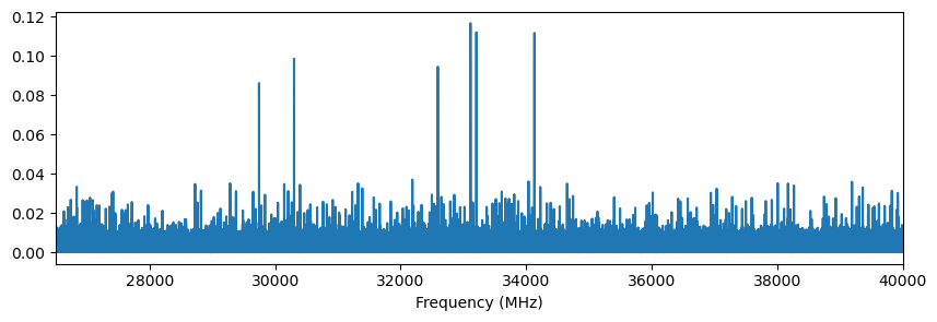
The CP-FTMW data are wrapped in a BCFTMW object accessible as BCExperiment.ftmw. For a single-FID acquisition the cumulative final FID is loaded with BCFTMW.get_fid(), returning a BCFid. The BCFid.ft() method computes the Fourier transform of that FID:

x, y = exp.ftmw.get_fid().ft()

fig, ax = plt.subplots(figsize=(10, 3))
ax.plot(x, y)
ax.set_xlabel('Frequency (MHz)')
ax.set_xlim(26500, 40000)

(26500.0, 40000.0)

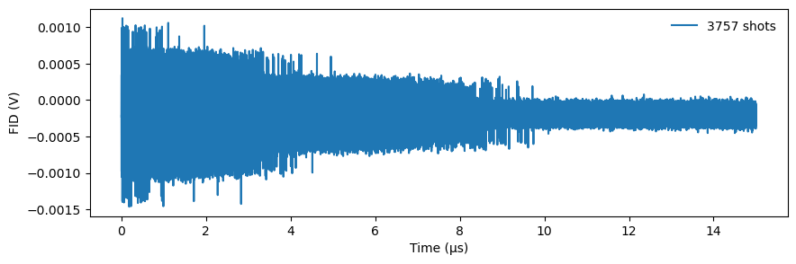
The FID itself can also be inspected. BCFid.y() returns the FID voltage array; BCFid.xy() returns the time array as well, in seconds by default. The units= keyword rescales the time axis. The chirp in this acquisition takes place from roughly 0.75 to 3.75 μs.

fid = exp.ftmw.get_fid()

fidx, fidy = fid.xy(units='us')
fig, ax = plt.subplots(figsize=(10, 3))
ax.plot(fidx, fidy, label=f'{int(fid.shots)} shots')
ax.set_xlabel('Time (μs)')
ax.set_ylabel('FID (V)')
ax.legend(frameon=False)

<matplotlib.legend.Legend at 0x7ff495c378c0>

fidy is a 2D numpy array. The second axis is the frame number; this acquisition has a single frame, but a multi-record acquisition would have more. A single frame can be selected by slicing (e.g. fidy[:, 3]).

fidy.shape

(750000, 1)

The contents of fidparams.csv are available as the fidparams attribute of BCFTMW. The sideband column is recorded by Blackchirp 2.0 as the enum name (UpperSideband / LowerSideband); older fixtures wrote the integer value 0 / 1. Either form works transparently — BCFid.is_lower_sideband() accepts both.

exp.ftmw.fidparams

	spacing	probefreq	vmult	shots	sideband	size
index
0	2.000000e-11	40960	0.000391	3757	LowerSideband	750000
1	2.000000e-11	40960	0.000391	1197	LowerSideband	750000
2	2.000000e-11	40960	0.000391	2398	LowerSideband	750000
3	2.000000e-11	40960	0.000391	3598	LowerSideband	750000

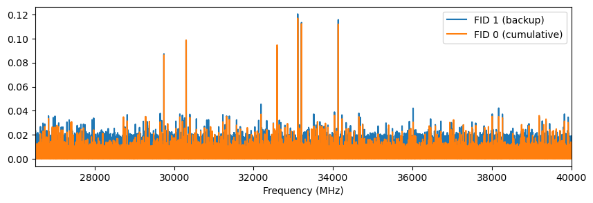
This experiment contains four FIDs: FID 0 is the final cumulative set, and FIDs 1, 2, 3 are intermediate backups taken during the acquisition. BCFTMW.get_fid() takes an optional FID number, so we can compare an early backup with the cumulative FID:

x_backup, y_backup = exp.ftmw.get_fid(1).ft()
fig, ax = plt.subplots(figsize=(10, 3))
ax.plot(x_backup, y_backup, label='FID 1 (backup)')
ax.plot(x, y, label='FID 0 (cumulative)')
ax.set_xlabel('Frequency (MHz)')
ax.set_xlim(26500, 40000)
ax.legend()

<matplotlib.legend.Legend at 0x7ff495cb9090>

BCFid.ft() also accepts overrides for any of the FID processing settings used by the Blackchirp GUI. The defaults come from processing.csv, which is exposed as the proc dictionary of BCFTMW. Note that Blackchirp 2.0 records FidWindowFunction and FtUnits as enum names (BlackmanHarris, FtuV); both name and integer forms are accepted. Note also one behavioural difference from the Blackchirp GUI: in the Python module, points within AutoscaleIgnoreMHz of the probe frequency are zeroed in the FT to make plot autoscaling well-behaved. The GUI keeps those points but excludes them from its vertical-range computation.

exp.ftmw.proc

{'AutoscaleIgnoreMHz': '250',
 'FidEndUs': '15',
 'FidExpfUs': '2.5',
 'FidRemoveDC': 'false',
 'FidStartUs': '3',
 'FidWindowFunction': 'BlackmanHarris',
 'FidZeroPadFactor': '1',
 'FtUnits': 'FtuV'}

BCFid.ft() allows any of these settings to be overridden:

help(fid.ft)

Help on method ft in module blackchirp.bcfid:

ft(
    *,
    start_us: 'float' = None,
    end_us: 'float' = None,
    winf: 'str' = None,
    zpf: 'int' = None,
    rdc: 'bool' = None,
    expf_us: 'float' = None,
    autoscale_MHz: 'float' = None,
    units_power: 'int' = None,
    frame: 'int' = None,
    freq_units: 'str' = 'MHz'
) -> 'tuple[np.ndarray, np.ndarray]' method of blackchirp.bcfid.BCFid instance
    Compute the Fourier transform of the FID

    By default, this computes the FT for each frame in the FID using the settings
    stored in the proc dictionary. This behavior can be overridden by specifying
    any combination of the keyword arguments.

    Args:
        start_us: Starting time, in μs. Points at earlier times are set to 0.
        end_us: Ending time, in μs. Points at later times are set to 0.
        winf: Window function name. One of ``None``, ``Bartlett``,
            ``Blackman``, ``BlackmanHarris``, ``Hamming``, ``Hanning``,
            ``KaiserBessel``. May also be passed in any form accepted by
            `scipy.signal.get_window <https://docs.scipy.org/doc/scipy/reference/generated/scipy.signal.get_window.html>`_
            — tuples and arbitrary names are forwarded directly.
        zpf: Zero-padding factor (positive integer). If nonzero, the FID is
            padded with zeroes until its length reaches the next power of 2,
            Then, its length is further extended by 2\*\*zpf.
        rdc: If true, the average of the FID is subtracted before the FT is
            computed.
        expf_us: Time constant for an exponential decay filter, in μs.
        autoscale_MHz: Range of FT points to set to 0, relative to the Downconversion
            LO frequency. Useful for suppressing noise near DC.
        units_power: FT is scaled by 10\*\*units_power. For μV units, set
            units_power=6. May also be specified in ``processing.csv`` as
            an enum name (``FtV`` / ``FtmV`` / ``FtuV`` / ``FtnV``) or
            as the corresponding integer.
        frame: Apply FT to only the specified frame.
        freq_units: Units for the returned frequency array. One of
            ``"Hz"``, ``"kHz"``, ``"MHz"`` (default), ``"GHz"``,
            ``"THz"``. ``start_us``, ``end_us``, ``expf_us``, and
            ``autoscale_MHz`` are interpreted in their declared
            units regardless of this choice.

    Returns:
        Frequency array (in ``freq_units``), Intensity array.

    Raises:
        ValueError: If ``winf`` is a string that does not match a known
            window-function name, if the ``FidWindowFunction`` value
            stored in ``processing.csv`` is unrecognised, if the
            ``FtUnits`` value is unrecognised, or if ``freq_units``
            is not a recognised frequency-unit string.

    Examples:
        Assuming a BCFid object named ``fid``::

            #default FT calculation
            x,y = fid.ft()

            #override some processing settings
            x,y = fid.ft(start_us=3.0,rdc=False,units_power=3)

            #compute ft for only frame 3 (assuming the number of frames is >=4)
            x,y = fid.ft(frame=3)

            #average all frames, then apply a custom window function
            fid.average_frames()
            p = 1.5
            sigma = len(fid)//5
            x,y = fid.ft(winf=('general_gaussian',p,sigma))

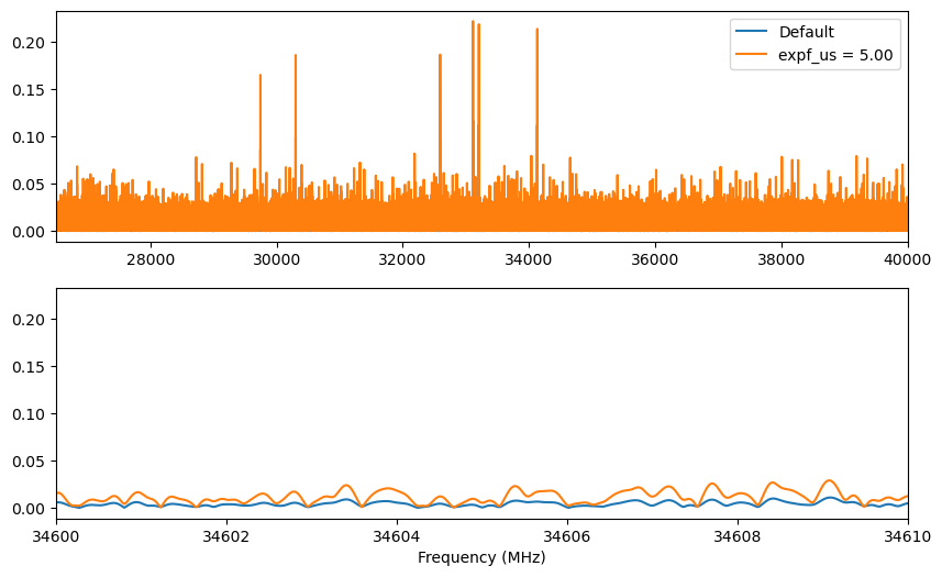
For example, override the exponential filter time constant and compare with the default settings:

expf = 5.0
x_filt, y_filt = exp.ftmw.get_fid().ft(expf_us=expf)

fig, axes = plt.subplots(2, 1, figsize=(10, 6))
for ax in axes:
    ax.plot(x, y, label='Default')
    ax.plot(x_filt, y_filt, label=f'expf_us = {expf:.2f}')
axes[0].set_xlim(26500, 40000)
axes[1].set_xlim(34600, 34610)
axes[0].legend()
axes[1].set_xlabel('Frequency (MHz)')

Text(0.5, 0, 'Frequency (MHz)')

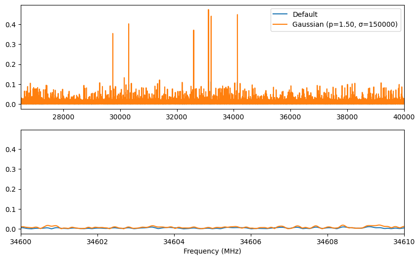
The Python module accepts a wider range of window functions than the GUI. The winf argument can be any value supported by `scipy.signal.get_window <https://docs.scipy.org/doc/scipy/reference/generated/scipy.signal.get_window.html>`__. For example, a generalized Gaussian window with explicit p and σ parameters is passed as a tuple:

p = 1.5
sigma = len(fid) // 5
x_win, y_win = fid.ft(winf=('general_gaussian', p, sigma))

fig, axes = plt.subplots(2, 1, figsize=(10, 6))
for ax in axes:
    ax.plot(x, y, label='Default')
    ax.plot(x_win, y_win, label=f'Gaussian (p={p:.2f}, σ={int(sigma)})')
axes[0].set_xlim(26500, 40000)
axes[1].set_xlim(34600, 34610)
axes[0].legend()
axes[1].set_xlabel('Frequency (MHz)')

Text(0.5, 0, 'Frequency (MHz)')

Like the FID, the FT y array is 2-D, with the second axis indexing the frame. By default, the FT is applied to all frames; pass frame=N to restrict it to one. The freq_units= keyword rescales the returned frequency axis to Hz, kHz, MHz, GHz, or THz.

y.shape

(1048577, 1)