Single LIF Example
Note: This notebook currently runs against synthetic data captured with Blackchirp 2.0 against its built-in virtual hardware. A refresh using real instrument data is planned and will land here without any change to the surrounding narrative or API surface.
This notebook walks through the LIF surface of the Blackchirp Python module against a small Blackchirp 2.0 fixture shipped with the source tree (python/example-data/v2-lif-ref/). It is a partial 6 × 6 (laser × delay) scan with a reference channel enabled. The acquisition was stopped before the full grid completed, so several scan points are missing — useful for exercising the missing-point handling on BCLIF.delay_slice, BCLIF.laser_slice, and BCLIF.image.
The package is on PyPI (pip install blackchirp); the recommended import style is from blackchirp import *. Matplotlib is imported for visualization but is not a runtime dependency of the blackchirp package itself.
[1]:
from blackchirp import *
from matplotlib import pyplot as plt
import numpy as np
Loading and Inspecting an Experiment
Pass BCExperiment the path to the experiment folder. When the folder contains a lif/ subdirectory, a BCLIF is constructed and exposed as exp.lif.
[2]:
ls example-data/v2-lif-ref/
auxdata.csv   header.csv  log.csv         version.csv
hardware.csv  lif/        objectives.csv
[3]:
exp = BCExperiment('./example-data/v2-lif-ref/')
exp.lif
[3]:
<blackchirp.bclif.BCLIF at 0x7f146339cc20>
BCLIF reads the scan-axis configuration from the LifConfig rows in header.csv at construction time. The delay_axis and laser_axis accessors return the full sample arrays together with their units strings:
[4]:
delays, delay_units = exp.lif.delay_axis()
lasers, laser_units = exp.lif.laser_axis()
delays, delay_units, lasers, laser_units
[4]:
(array([200., 210., 220., 230., 240., 250.]),
 'μs',
 array([280., 281., 282., 283., 284., 285.]),
 'nm')
The lifparams attribute is the index of acquired scan points. Only rows present in lifparams.csv were actually written to disk; any (lIndex, dIndex) combination not in this table was never acquired.
[5]:
exp.lif.lifparams
[5]:
| lIndex | dIndex | shots | lifsize | refsize | spacing | lifymult | refymult | |
|---|---|---|---|---|---|---|---|---|
| 0 | 0 | 0 | 20 | 10000 | 10000 | 8.000000e-10 | 0.001953 | 0.000391 |
| 1 | 1 | 0 | 20 | 10000 | 10000 | 8.000000e-10 | 0.001953 | 0.000391 |
| 2 | 2 | 0 | 20 | 10000 | 10000 | 8.000000e-10 | 0.001953 | 0.000391 |
| 3 | 0 | 1 | 20 | 10000 | 10000 | 8.000000e-10 | 0.001953 | 0.000391 |
| 4 | 1 | 1 | 20 | 10000 | 10000 | 8.000000e-10 | 0.001953 | 0.000391 |
| 5 | 2 | 1 | 6 | 10000 | 10000 | 8.000000e-10 | 0.001953 | 0.000391 |
| 6 | 0 | 2 | 20 | 10000 | 10000 | 8.000000e-10 | 0.001953 | 0.000391 |
| 7 | 1 | 2 | 20 | 10000 | 10000 | 8.000000e-10 | 0.001953 | 0.000391 |
| 8 | 0 | 3 | 20 | 10000 | 10000 | 8.000000e-10 | 0.001953 | 0.000391 |
| 9 | 1 | 3 | 20 | 10000 | 10000 | 8.000000e-10 | 0.001953 | 0.000391 |
| 10 | 0 | 4 | 20 | 10000 | 10000 | 8.000000e-10 | 0.001953 | 0.000391 |
| 11 | 1 | 4 | 20 | 10000 | 10000 | 8.000000e-10 | 0.001953 | 0.000391 |
| 12 | 0 | 5 | 20 | 10000 | 10000 | 8.000000e-10 | 0.001953 | 0.000391 |
| 13 | 1 | 5 | 20 | 10000 | 10000 | 8.000000e-10 | 0.001953 | 0.000391 |
The default integration gates and waveform-filter settings live in lif/processing.csv and are exposed as the proc dictionary. These are the same controls that the LIF tab in the Blackchirp GUI exposes.
[6]:
exp.lif.proc
[6]:
{'LifGateEndPoint': 1421,
 'LifGateStartPoint': 500,
 'LowPassAlpha': 0.0,
 'RefGateEndPoint': 300,
 'RefGateStartPoint': 100,
 'SavGolEnabled': False,
 'SavGolPoly': 3,
 'SavGolWindow': 11}
Inspecting a Single Trace
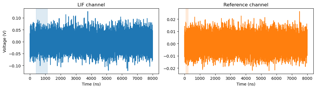
Per-point traces are loaded lazily via BCLIF.get_trace(l_index, d_index). For this fixture, (l=0, d=0) is the lower-left corner of the scan. The returned BCLifTrace exposes the LIF waveform (lif()), the optional reference waveform (ref()), and the time axis (x() or xy()).
[7]:
trace = exp.lif.get_trace(l_index=0, d_index=0)
trace.shots, trace.lifsize, trace.refsize, trace.spacing
[7]:
(20, 10000, 10000, 8e-10)
Plot the raw LIF and reference channels side-by-side. The integration gates from processing.csv are overlaid as shaded regions to show where BCLifTrace.integrate will sum:
[8]:
x_ns = trace.x(units='ns')
lif_y = trace.lif()
ref_y = trace.ref()

lif_gate = (exp.lif.proc['LifGateStartPoint'], exp.lif.proc['LifGateEndPoint'])
ref_gate = (exp.lif.proc['RefGateStartPoint'], exp.lif.proc['RefGateEndPoint'])

fig, (ax_l, ax_r) = plt.subplots(1, 2, figsize=(11, 3.2), sharey=False)
ax_l.plot(x_ns, lif_y, color='C0')
ax_l.axvspan(x_ns[lif_gate[0]], x_ns[lif_gate[1]], color='C0', alpha=0.15)
ax_l.set_title('LIF channel')
ax_l.set_xlabel('Time (ns)')
ax_l.set_ylabel('Voltage (V)')
ax_r.plot(x_ns, ref_y, color='C1')
ax_r.axvspan(x_ns[ref_gate[0]], x_ns[ref_gate[1]], color='C1', alpha=0.15)
ax_r.set_title('Reference channel')
ax_r.set_xlabel('Time (ns)')
fig.tight_layout()
Smoothing and Integration
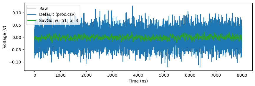
BCLifTrace.smooth applies the IIR low-pass filter followed by the Savitzky-Golay smoother that the GUI uses. Both stages follow processing.csv by default; pass low_pass=..., savgol=..., or any of the named parameter overrides to deviate. To see the effect of an aggressive Savitzky-Golay window, force savgol=True with a wider window:
[9]:
raw = trace.lif()
smoothed_default = trace.smooth()  # follows processing.csv
smoothed_strong = trace.smooth(savgol=True, savgol_window=51, savgol_poly=3)

fig, ax = plt.subplots(figsize=(10, 3))
ax.plot(x_ns, raw, color='0.7', label='Raw')
ax.plot(x_ns, smoothed_default, color='C0', label='Default (proc.csv)')
ax.plot(x_ns, smoothed_strong, color='C2', label='SavGol w=51, p=3')
ax.set_xlabel('Time (ns)')
ax.set_ylabel('Voltage (V)')
ax.legend()
[9]:
<matplotlib.legend.Legend at 0x7f13bd067e00>
BCLifTrace.integrate runs the same filter chain and then takes a trapezoidal sum in sample-index space between the LIF gate endpoints. With a reference channel present (as here), the return value is the dimensionless ratio of LIF integral over reference integral. To get the unratioed LIF integral instead, override the reference gate so it collapses to zero (or use the v2-lif-noref/ fixture, which has no reference channel at all).
[10]:
integral_default = trace.integrate()
integral_wide_lif = trace.integrate(lif_start=400, lif_end=1600)
integral_default, integral_wide_lif
[10]:
(7.926510330398397, 11.893470490802894)
Aggregating Helpers
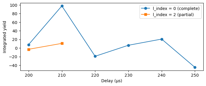
BCLIF.delay_slice(l_index) integrates every present trace at one laser index and returns (delay_axis, integrals) arrays sized against the full delay axis. Missing scan points are filled with np.nan by default. For l=2 in this fixture, only two delay points were acquired — the rest come back as NaN:
[11]:
delays_axis, integrals_l0 = exp.lif.delay_slice(l_index=0)
delays_axis, integrals_l2 = exp.lif.delay_slice(l_index=2)

fig, ax = plt.subplots(figsize=(8, 3))
ax.plot(delays_axis, integrals_l0, marker='o', label='l_index = 0 (complete)')
ax.plot(delays_axis, integrals_l2, marker='s', label='l_index = 2 (partial)')
ax.set_xlabel(f'Delay ({delay_units})')
ax.set_ylabel('Integrated yield')
ax.legend()
[11]:
<matplotlib.legend.Legend at 0x7f1461800f50>
Pass fill=0.0 (or any other numeric value) to substitute the missing positions with that value rather than NaN. This is convenient when downstream code (or matplotlib) does not handle NaN gracefully:
[12]:
_, integrals_l2_zero = exp.lif.delay_slice(l_index=2, fill=0.0)
integrals_l2_zero
[12]:
array([-2.92994452, 10.77452153,  0.        ,  0.        ,  0.        ,
        0.        ])
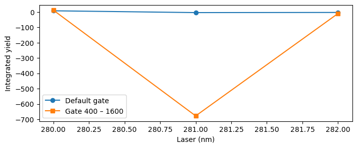
BCLIF.laser_slice(d_index) is the symmetric helper across the laser axis. Override the gate positions per call to integrate over a different sample range without modifying processing.csv:
[13]:
lasers_axis, integrals_d0 = exp.lif.laser_slice(d_index=0)
_, integrals_d0_wide = exp.lif.laser_slice(d_index=0, lif_start=400, lif_end=1600)

fig, ax = plt.subplots(figsize=(8, 3))
ax.plot(lasers_axis, integrals_d0, marker='o', label='Default gate')
ax.plot(lasers_axis, integrals_d0_wide, marker='s', label='Gate 400 – 1600')
ax.set_xlabel(f'Laser ({laser_units})')
ax.set_ylabel('Integrated yield')
ax.legend()
[13]:
<matplotlib.legend.Legend at 0x7f1461689450>
Full 2D Image
BCLIF.image() integrates every present scan point into a 2-D array of shape (delay_points, laser_points). The same fill= keyword controls the missing-point value. Plot both forms side-by-side to make the difference visible: NaN cells are drawn as the colormap’s background by pcolormesh, while fill=0.0 makes them part of the color range.
[14]:
delays_img, lasers_img, image_nan = exp.lif.image()
_, _, image_zero = exp.lif.image(fill=0.0)
image_nan.shape, image_zero.shape
[14]:
((6, 6), (6, 6))
[15]:
fig, (ax_n, ax_z) = plt.subplots(1, 2, figsize=(11, 4), sharex=True, sharey=True)
mesh_n = ax_n.pcolormesh(lasers_img, delays_img, image_nan, shading='nearest', cmap='viridis')
ax_n.set_title('fill=np.nan (default)')
ax_n.set_xlabel(f'Laser ({laser_units})')
ax_n.set_ylabel(f'Delay ({delay_units})')
fig.colorbar(mesh_n, ax=ax_n, label='Integrated yield')
mesh_z = ax_z.pcolormesh(lasers_img, delays_img, image_zero, shading='nearest', cmap='viridis')
ax_z.set_title('fill=0.0')
ax_z.set_xlabel(f'Laser ({laser_units})')
fig.colorbar(mesh_z, ax=ax_z, label='Integrated yield')
fig.tight_layout()
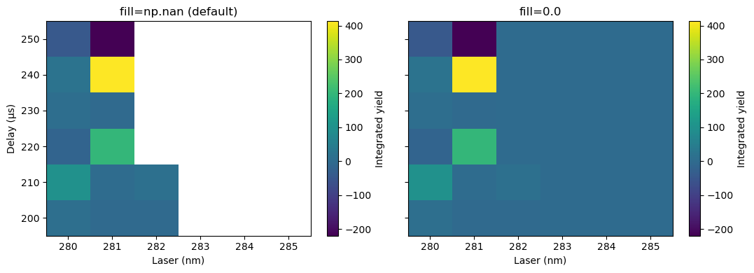
pcolormesh works well when the scan grid is at least 2 × 2. When one of the scan axes has only a single point, shading='flat' (the default) collapses the entire row or column to zero quads and the plot appears empty. shading='nearest' (used above) handles that case but still requires you to pass the axis arrays as cell centers.
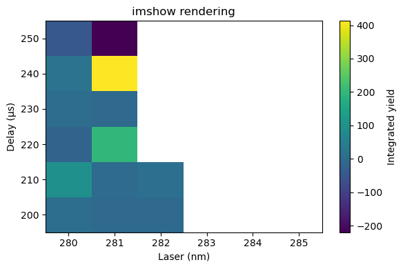
An alternative is imshow, which always draws one pixel per array element regardless of axis length. It assumes a uniformly spaced grid — which the LIF delay and laser axes always are — and takes the data extent through the extent= keyword. aspect='auto' is essential, otherwise a (1, N) image is rendered as a sliver one pixel tall; origin='lower' flips the y-axis so increasing delay points upward as expected.
[16]:
delay_step = exp.lif.delay_step
laser_step = exp.lif.laser_step
extent = (
    lasers_img[0] - laser_step / 2,
    lasers_img[-1] + laser_step / 2,
    delays_img[0] - delay_step / 2,
    delays_img[-1] + delay_step / 2,
)

fig, ax = plt.subplots(figsize=(6, 4))
im = ax.imshow(
    image_nan,
    extent=extent,
    origin='lower',
    aspect='auto',
    interpolation='nearest',
    cmap='viridis',
)
ax.set_title('imshow rendering')
ax.set_xlabel(f'Laser ({laser_units})')
ax.set_ylabel(f'Delay ({delay_units})')
fig.colorbar(im, ax=ax, label='Integrated yield')
fig.tight_layout()
Processing overrides forwarded to image() apply uniformly to every integrated point, so a single call sweeps the full scan grid through any alternative gate or filter setting:
[17]:
_, _, image_wide = exp.lif.image(lif_start=400, lif_end=1600)
image_wide
[17]:
array([[  11.89347049, -677.37704918,   -9.88711134,           nan,
                  nan,           nan],
       [ 127.9601227 ,  -13.45579911,   11.55502392,           nan,
                  nan,           nan],
       [ -16.35057208,   31.16666667,           nan,           nan,
                  nan,           nan],
       [   7.12971133,    3.88729112,           nan,           nan,
                  nan,           nan],
       [  52.37049415,  363.94012945,           nan,           nan,
                  nan,           nan],
       [-110.82105719, -414.69733656,           nan,           nan,
                  nan,           nan]])